How Convolutional Neural Networks Work.

Convolutional Neural Networks also called CNNs or ConvNets have been pivotal in Deep Learning excelling in classifying images. When working with CNNs it is important to develop an intuitive understanding of how they work. I will attempt to describe how I understand them based on Brandon Rohrer’s awesome video. Its worth the watch. Credit goes to Brandon for all the images which did a thorough job of demonstrating how CNNs work. I just added my small twist to it but he provides the best CNN explanation I have encountered so far.

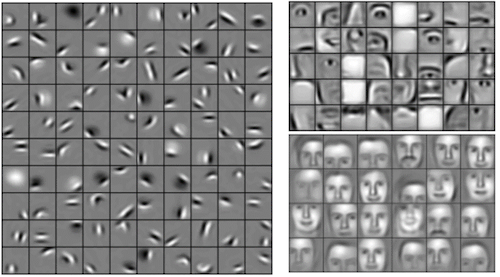
If you feed CNNs with pictures of faces they will learn about edges, bright and dark spots etc and because they are multilayer, in a subsequent layer they can learn about recognizable things like eyes,noses or mouths. In another layer they may learn about things that resemble faces.

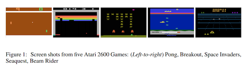
CNNs can also learn to play video games by forming patterns of the pixels as they appear on the screen and learning the best action to take when they identify a certain pattern.

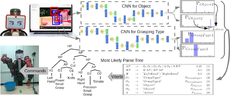
More interestingly, if you get some CNNs and set them to watch YouTube videos, one can learn about objects and the other can learn types of grasps by again identifying patterns. When this is combined with some execution software, It can enable a robot learn to cook by watching YouTube videos

From the above examples. It is clear that CNNs are powerful and they are almost like magic. However, how they work is really based on basic ideas which are applied cleverly.

Lets illustrate this by taking a simple example of a CNN.

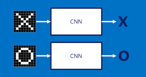
Our CNN takes an image which is a two-dimensional array of pixels where each square in this array is either light or dark like a checkerboard. The CNN then decides whether it is an image of an X or an O.

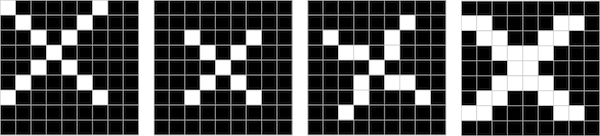
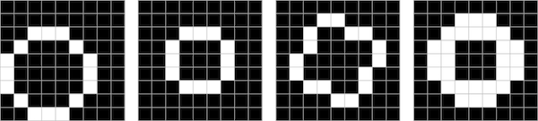
We would like our CNN to be able to identify an X or 0 whether they are slightly rotated, thicker, scaled down etc.

This is very easy for a human but not so straigt forward for a computer. A computer really only sees a bunch of 1’s and -1’s where 1 is a white pixel and -1 is a black pixel

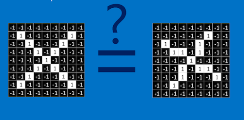
A computer has to go pixel by pixel to determine if there is a match. It will notice that some pixels match but most don’t.

A computer therefore will determine that the images are not equal.

Conversely, a CNN matches pieces of the image rather attempting to match the whole image

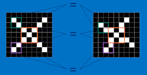
When a CNN matches pieces of the image called features. It becomes much more clearer that these images are equal.

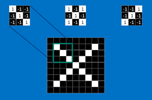
These features are like mini-images and they match common parts of the image for example an X has diagonal lines and a crossing which capture most of the details about an X. If you choose the right feature and fit it in the right place, it matches the image.

To take this a step further, we look at the Math behind matching the features. This is called Filtering

Filtering consists of four steps

• Line up the feature and the image patch
• Multiply each image pixel by the corresponding feature pixel
• Add them up
• Divide by the total number of pixels in the feature

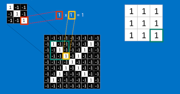
We can see from above that if we multiply every corresponding pixel of the feature with a matching image patch we get 1 throughout. We add all this pixels together i.e(1+1+1+1+1+1+1+1+1=9) divide by the total number pixels which is 9 and we get 1. To keep track of where this feature is we put 1 which means it matched

This is filtering.

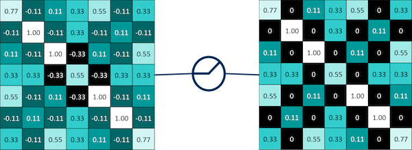
We can move this feature to another position and perform filtering again

We can see that in areas the pixels don’t match we will get a -1 because (1x-1 = -1). In our new position we will get two -1’s. When we add the pixels up (1+1-1+1+1+1-1+1+1=5) and divide by 9 we will get 0.55

We then record the 0.55 in the position where the feature doesn’t match.

Therefore by moving our filter around different positions of the image, we find different values for how well that feature matches the position or how well it is represented at that position. It essentially becomes a map of where the feature occurs.

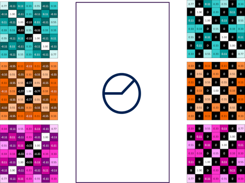
By moving this feature around to every possible position we do Convolution which is repeated application of this filter. We get a map of where this feature occurs.

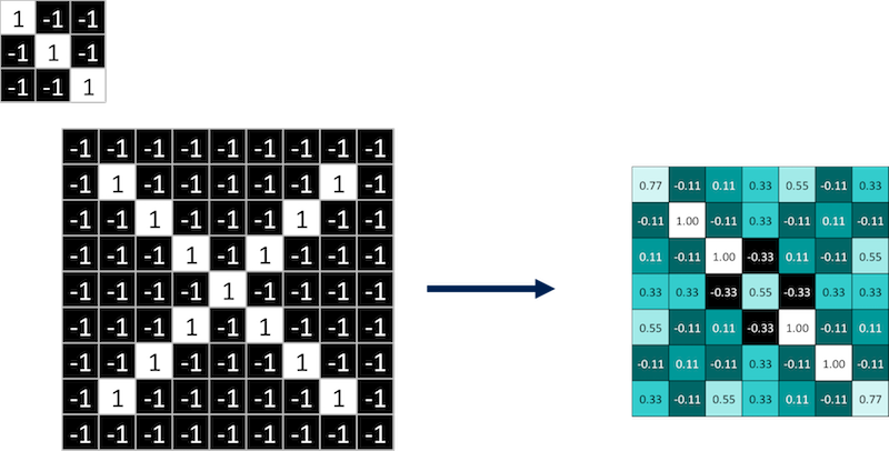
If we look at the map we can see that our feature which is a diagonal line from left to right matches similar positions in our map. All the high numbers are along the diagonal from left to right in our filtered image which implies that the feature matches along that diagonal much better than anywhere else in the image.

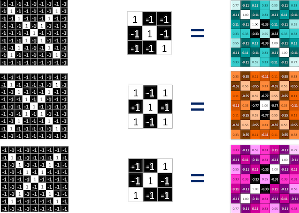
This process is repeated for every feature and for each feature we get a map which is consistent with what we would expect based on what we know about X and where we know our features will match.

The process of convolving an image with a bunch of filters creates a stack of filtered images which is called a convolution layer. This layer can be stacked with other operations. Therefore in convolution an image becomes a stack of filtered images.

Convolution is the first trick we use. Our next trick is called Pooling which is shrinking the image stack. Pooling consists of four steps just like filtering which are

• Pick a window size(usually 2 or 3 pixels)
• Pick a stride (usually 2 pixels)
• Walk your window in strides across your filtered images.
• From each window, take the maximum value.

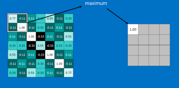
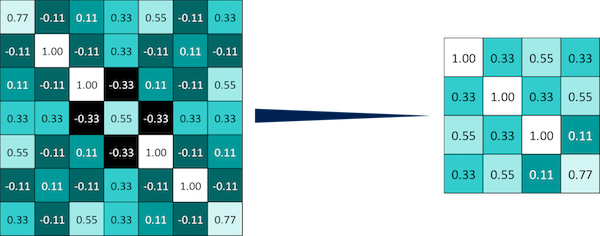
We repeat this process across the whole image and in the end we have a smaller pattern which has retained most of the important information from the previous pattern i.e we can still see our diagonal from left to right. Instead of a 7x7 pixel image we now have a 4x4 pixel image.

Pooling has important advantages when it comes to shrinking images particulary when you have large images. Pooling is also not concerned about the location of the maximum value in the window making it less sensitive to position. Regardless of where the feature is i.e if its slight rotated etc. Pooling will pick it up.

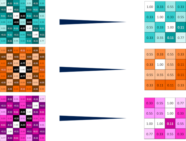
Max Pooling is carried out with all stacks of filtered images such that the stack of images becomes a stack of smaller images.

The third trick we use is called Normalization which is basically preventing the learned values from going to zero or going to infinity. During normalization we change all the values that are negative to zero.

We use computational units called Rectified Linear Units (ReLUs). All they do is step through all the negative values and convert them to zero.

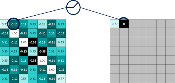
This new stack of images with no negative values becomes our ReLU layer.

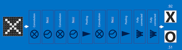
The magic of CNNs happens when we begin to stack these layers on top of each other where the input of one layer becomes the output of another layer.

What goes into and out of each layer is an array of pixels which makes it easy to stack the layers nicely.

We can stack these layers many times i.e deep stacking where each image gets more filtered as it goes through convolution layers and smaller as it goes through pooling layers

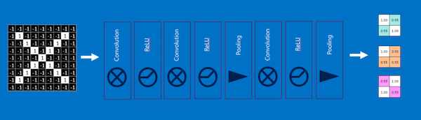
Our final layer is called the Fully Connected Layer where every value of the filtered images gets a vote on what the answer should be

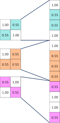
We connect each of values of our filtered images to one of the answers we are going to vote for. When we feed X into our CNN some of these values will be high and strongly imply that its an X and when feed O into our CNN some of these values will be high and also imply that its an O. The vote will depend on how strongly a value predicts X or O.

Therefore when we get a new input and want to determine whether its an X or an O. The input will go through our Convolution Layers, ReLU layers and Pooling layers and in the fully connected layer, we get a series of votes and based on the weights each value gets to vote with,an average vote is calculated.

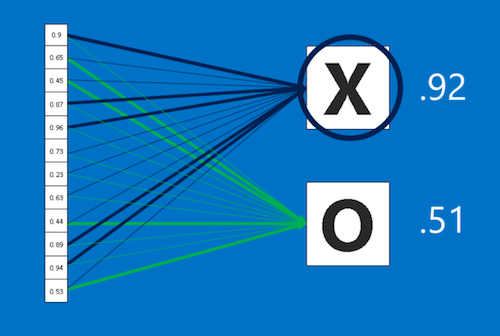
In the example above the inputs vote for an X with a strength of 0.92 and an O of strength 0.51. The CNN will therefore categorize the input as an X

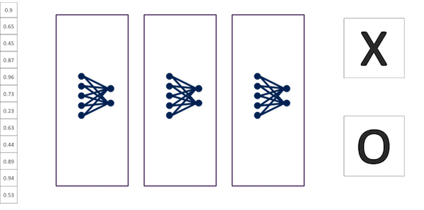
In the fully connected layer, a list of feature values becomes a list of votes and because they are similar to the feature values, they can also be stacked such that you have intermediate votes which are not the final votes. These are called hidden units and you can stack as many as you want. They always end up voting for an X or an O

Therefore when we put this altogether a two dimensional array of pixels becomes a set of votes for a category.

While we have presented a good intuitive way of understanding CNNs a lot of details have been left out. Where do the magic numbers come from? where did the features in the convolution layers come from? Where do the voting weights in the fully connected layers come from? etc.

The answer is a trick called Backpropagation. You don’t have to know any of them. They are learned by the Neural Network.

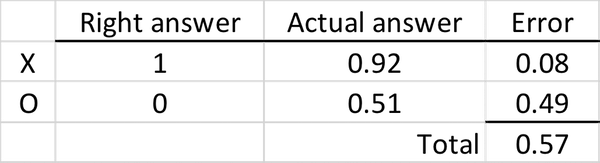
The fundamental principle of backpropagation is that the error(right answer - actual answer) in the final answer is used to determine how much the network adjusts.

This error signal drives a process called Gradient descent where each feature pixel and voting weight is adjusted up and down a bit to see how the error changes. Large errors lead to a large adjustment and small errors lead to a small adjustment. No error means no adjustment. It is analogous to sliding a ball slightly to the right or to the left on a hill and you want to find the direction where it goes downhill ( as you can see below down means the error is reducing hence the name “Gradient descent”). You want to go down to the very bottom of the Gradient where the error is the least.

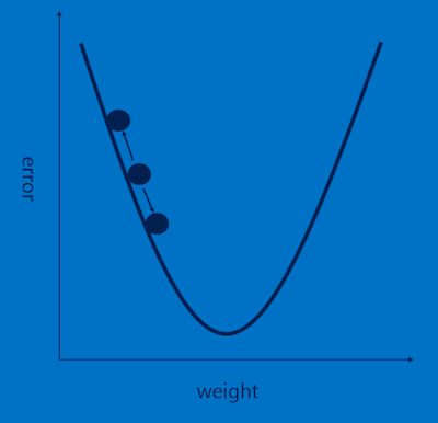
Doing this over lots of iterations helps all these values across the features and weights settle into a “minimum” where the network is performing as well as it can and any adjustment would lead to increase in the error.

There are things called Hyperparameters which a designer of a CNN model gets to chose. They are not learnt automatically. Think of them as knobs you can adjust.

In the convolution layer figuring out how many features should be used and the size of the features(pixels).

In the pooling layers we have to choose the window size and window stride

In the fully connected layer, choosing the number of hidden neurons.

All these must be chosen by the designer. In practice there are common ways that have been proved to be effective but in general there are no hard and fast rules when dealing with hyperparameters. Adjusting them comes mostly from intuition and experience. In fact most advances in CNNs come from finding novel ways of combining them.

In addition to this the designer has to decide how many of each type of layer and in what order the layers should be and for the extra curious which new layers can be created. These are all things people are playing with to try to eke out as much performance as possible from CNNs to address more challenging problems.

So far, we have been talking about images but we can use any 2 Dimensional or 3 Dimensional data as long as the data meets the criteria that things closer together are more closely related than things far away.

What this means is if for example we look at our image X. Two rows of pixels and two columns of pixels next to each other are more closely related than rows or columns that are far away.

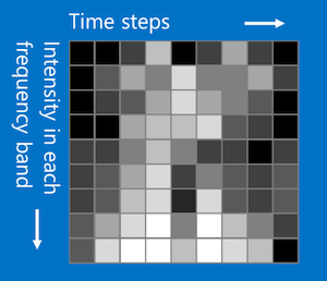
What we can we do for example for sound is to divide a sound signal into time steps and for each piece of time, the time step before and the time step after are more closely related than time steps that are far away and the order matters.

We can also divide the sound into different frequency bands like bass,midrange,treble etc and for the bands, those closer together are more related than those that are far away and the order matters.

The order mattering means the time steps and frequency bands must be in a specific order. If you change the order you will most likely lose the original sound.

Once you do this to sound it looks like an image and you can apply CNNs.

You can also do something similar with text where the position in the sentence becomes the column and the row is words in a dictionary.

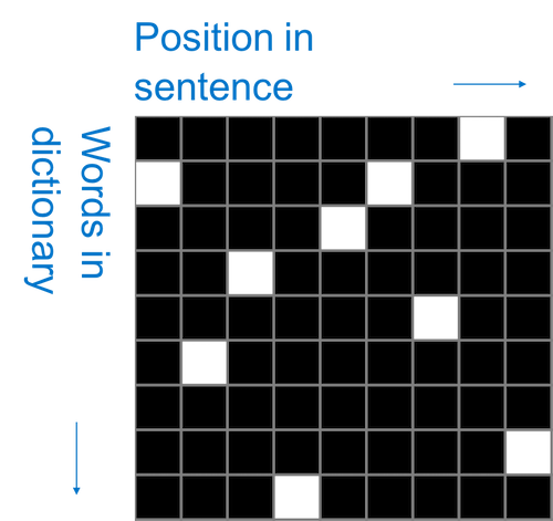
Its not really clear if order matters here because its not necessarily true that words in dictionary that are close to each other are related and therefore the trick is to take a window that spans the entire column from top to bottom and slide it left to right such that it captures all the words but only a few positions in the sentences at a time.

CNNs are awesome but they have limitations because they only capture local “spatial” patterns where spatial means that patterns that are next to each other matter. If the data can’t be made to look like an image they are not very useful. So basically as rule of thumb if data is as useful after swapping any of your columns with each other, then you can’t use Convolutional Neural Networks.

CNNs are therefore good at finding patterns and using them to classify images.

Thanks for sticking with the post to the end and I hope you have a clear idea of how CNNs work. Special thanks to Brandon Rohrer for his awesome video which this post is based on. The post is really meant to help me internalize the video and its purely Brandon’s work not mine. I hope it helps you too.